Configuration file formats
AtomEye works with atomistic configurations, the format of which should follow the general guidelines below from our experience:
- One file stores only one configuration. XMol XYZ's concatenated format is not recommended.
- For portability, the file should be in ASCII plain text that a human can read.
- There should minimally be chemical symbol designation for each atom and some representation for its position.
- It is recommended to define comment line in the format, and a configuration file should be self-explanatory with the aid of comments.
AtomEye currently supports the following formats:
PDB | standard CFG |
extended CFG
All configuration files can be
compressed by gzip / bzip2 and then fed directly
into AtomEye, which looks for magic number at the first few bytes, and
if found would automatically decompress it by calling shell
gzip/bzip2. In order to use this feature, the user must install
gzip/bzip2 executable in his shell PATH.
Standard or extended CFG formats are strongly
recommended over the PDB format for hassle-free
rendering by AtomEye. Among other things, standard or extended
CFG formats allow arbitrary numerical precision. Also, enforcing PBC
is quite a bit of work for the PDB format, but is
built-in in standard or extended CFG formats.
PDB examples:
DNA.pdb |
Nanotube8x3x1.pdb |
SiShuffle.pdb
In order to enforce periodic boundary condition (PBC) behavior in
AtomEye, one must insert the following two lines at the beginning of
the file:
A configuration file is considered to be in PDB format if there is
'.pdb' or '.PDB' in the filename.
The standard CFG format ensures seamless transition and
complete information passage from one MD simulation to the
other. Thus particle velocities must be specified, and
floating-point numbers are usually saved to the 16th significant
digit. Aside from an atom's position and velocity, properties such as
the local energy are deemed potential-dependent and therefore cannot
be specified in the standard format.
The shortcoming of the standard CFG format is its lack of
extensibility, and the filesize tends to be noticeably larger for very
large configurations (>200K atoms).
Standard CFG examples:
SiVacancy.cfg |
Si_screw_dipole.cfg |
Cu_NanoXtal.cfg.bz2
Take a look at SiVacancy.cfg. The format
consists of system specifications and atom specifications. The system
specifications are of the form 'tagname = value units', where
'tagname' and 'units' are fixed, and 'value' needs to be filled
in. Some tagnames are required, such as 'Number of particles',
'H0(1,1)' to 'H0(3,3)'. Some are optional, such as 'A', 'eta(1,1)',
'R'. A line starting with '#' is comment. Here the comments explain
the tags immediately above, which is a good habit.
The atom specifications are the rows above, one row for each atom,
with the meaning of each column entry explained in the comments. The
reduced coordinates s1,s2,s3 should be between 0 and 1. The Cartesian coordinates of the atoms can be determined
from the reduced coordinates as,
'A', 'R' are the lengthscale and ratescale of H0[][] and ds[]/dt,
respectively, which by default take the values Angstrom and
nanosecond^-1. They can be altered to manually dilate or heat up the
system. 'eta[][]' is the optional Lagrangian strain which is 0 by
default, using which we can apply an additional deformation on H0[][]
to get the actual box shape H[][]. These are amenities that
entry-level users can do without.
Extended CFG examples:
BubbleRaftBefore.cfg |
BubbleRaftAfter1.cfg
Extended CFG format addresses the problem of filesize and
extensibility. Velocity data is no longer required for the atoms, and
floating-point precision can be what one sees fit for the application
instead of the recommended 16 significant digits in case of the
standard CFG format. Also, atomic mass and chemical symbol are now
assigned on a block-by-block basis instead of on an atom-by-atom
basis. All standard CFG system tags are still valid in the extended
CFG format, with addition of the 'entry_count' keyword, whose
appearance determines whether this is standard or extended CFG format.
In above, 'entry_count = 11' means there are 11 entries per row for
an atom. To omit velocity data in rows, write '.NO_VELOCITY.' line
before the 'entry_count = 11' line. In this case because 11=3+8, we
must have 8 so-called auxiliary properties per atom. If on the
other hand '.NO_VELOCITY.' does not appear before 'entry_count = 11',
then the velocities (ds[]/dt in R) will be specified after s[] in each
row, and since 11=3+3+5, we will have only 5 auxiliary properties.
For AtomEye to know what these auxiliary properties are, so it can
provide the correct help information, one should also fill in
'auxiliary[i] = name [unitname]' lines, where 'i' runs from 0 to 8-1=7
here, 'name' is a single word for the property's name, and unitname is
the name of the unit in which the values are given. For example,
'auxiliary[3] = mises [GPa]' would mean that the fourth
auxiliary property, which is the 7th column (or the 10th column if
'.NO_VELOCITY.' clause is not given), are the von Mises stress
invariants in GPa.
Lastly, atomic mass and chemical symbol are now assigned on a
block-by-block basis. In the above file all atoms would be
1.000000 amu Ar, which is a pseudonym for soap bubble. Apparently this
format can save considerable space for monoatomic configuration. When
we have binary compounds, we can write,
Sometime it is more convenient to have the auxiliary properties in
a stand-alone '.aux' file, which can be patched to the current
application on-demand (press 'F11'). This file should look like,
This can be accomplished either with arrow keys or mouse
drag. Press Left, Right, Up, Down keys to rotate object as if you are
rolling a crystal ball with the object embedded in it. For in-plane
rotation, use Shift+Up (clockwise) and Shift+Down (counter-clockwise).
The angle of rotation corresponding to one keystroke is controlled by
the gearbox value multiplied by
pi. Therefore, at gear-9 corresponding to gearbox value of 0.5, each
keystroke will flip the object by pi/2, which comes in handy when
viewing large configurations.
One can also rotate the viewport by pressing left button and drag
the mouse. The "crystal ball" can be imagined as being hinged at the
viewport center and whose diameter is somewhat smaller than the
viewport. If the pointer should fall onto the crystal ball's surface,
the rotation follows a geodesic path connecting A and B on the ball's
surface. On the other hand, if the pointer falls outside of the ball,
then dragging the mouse will just rotate the object
clockwise/counter-clockwise in-plane.
It can be foreseen that when the configuration is large, it is much
more efficient to rotate the viewport than to rotate the object. In
fact, contrary to what the heading suggests, this is how I
implement the rotation. To get the correct look and feel, one must
also translate the viewport after the rotation. It is done by
the following rule: we stipulate that there exists a location in space
whereby the combined effect of rotation and translation would not
change its subjective position with respect to the
viewport. This location is called the anchor, named so because
when we "rotate the object", it appears to be hinging on the
anchor. Please visit anchor control to see
how to change the anchor position.
At the start of a session, the anchor is taken to be the center of
the box, so the object appears to be hinged at the box center if
rotated. This state can be recovered whenever 'w' is pressed.
On the other hand, right-clicking on an atom transfers the anchor
to that atom's position. This allows a streamlined right click + drag
action that pulls the viewport closer to any atom you want to see in
detail. Also, once you right-clicked on an atom, ensuing rotations
will be hinged on that atom, which is convenient for studying local
atomic arrangements.
If you are in the bond mode, then
right-clicking on a bond will also set the anchor position to the bond
center.
Press 'a' to shift the viewport so the anchor is seen right at the
middle of the viewport.
Press 'b' to toggle whether to draw bonds or not. To change
the bonding cutoff between two species of atoms, visit
Cutoff Control.
Press 'Tab' to toggle between parallel and perspective projection
rendering methods. Parallel projection is a limiting case of
perspective projection, where the viewpoint is very far away from the
object but the view angle is also
turned very small. It is useful for discerning atomic rows and planes.
Press 'PageUp' to increase atom radii and 'PageDown' to decrease
atom radii rendered on screen by a common factor. The rate of change
is controlled by the gearbox.
Press 'Home' to increase bond radius and 'End' to decrease bond radius
drawn on the screen. The rate of change is controlled by the gearbox.
Press 'i' to toggle wireframe mode that determines how to render
the PBC box. You have the freedom to select no wireframe,
monochromatic wireframe, RGB wireframe, and so on. In the case of the
RGB wireframe, the three axes correspond to (s1,0,0), (0,s2,0),
(0,0,s3), respectively; the point they meet corresponds to the origin
(0,0,0).
Press 'r' for cutoff control, which decides how close two atoms
need to be with each other to be considered nearest neighbor (if they
are, then each atom's coordination number will be increased by 1, and
a bond will be drawn between them if under the bond mode).
You will be first inquired about which two species. For example, if
you want to change the cutoff distance between silicon and carbon,
then you should enter "Si C" and press enter. Then, with each
Ctrl+Home/Ctrl+End, the cutoff distance will be increased/decreased;
the rate of change is controlled by the gearbox. When you are satisfied, you should
press 'r' again to close the change, so you can't modify two pairing
types at the same time.
Sometimes too much rotation is a bad thing, and you want the
viewframe upright again just like at the beginning. Press 'u'.
Right click on an atom to display relevant information about it in
the xterm. This will also set the anchor
to this atom.
Right-clicking on a bond will display information about this
bond. This will set the anchor to the bond
center.
AtomEye remembers the last four atoms that you have clicked on.
Right click in the window and drag mouse to pull
closer. Alternatively, use IMWheel (or Ctrl+IMWheel for quicker
action) to pull viewport closer/away from the anchor. If you click on
an atom, that atom will automatically become the anchor. If you click on a bond, the bond
center will also become the anchor.
Ctrl+Left, Ctrl+Right, Ctrl+Up, Ctrl+Down will shift the object in
plane. Ctrl+Shift+Up will send the object further from viewport,
Ctrl+Shift+Down will pull it closer.
Press numeral keys '0' to '9', and the gearbox value will be
switched to,
Press 'k' to toggle coordination number coloring. Coordination
number is an empirical measure of how many nearest neighbors (could be
of various species) there are for a particular atom. The definition of
"nearest neighbors" can be changed by cutoff
control.
To clearly see defect cores, you often need to remove the perfectly
coordinated atoms. This is done in Make
Atoms Invisible.
Meta+g will color-encode the atoms according to
their local von Mises shear strain
invariant. Shift+g will toggle the flag controlling whether to
subtract off the system-averaged strain tensor or not before computing
the invariant; the default is no. The controls of colormap,
visibilities etc. are identical to that of auxiliary properties coloring.
Meta+h will color-encode the atoms according to
their central symmetry parameter
c's. Shift+h will prompt the user to change the maximum number
of neighbors M used in the computation; the default being the
most popular coordination number of the configuration rounded
even. The controls of colormap, visibilities etc. are identical to
that of auxiliary properties
coloring.
Because calculating the central symmetry parameters requires a neighborlist without pairwise saving, it
is not calculated by default when the configuration is loaded, but
only computed after Meta+h is pressed. c is
between [0,1], and its average is usually less than 0.5 even for
amorphous structures. An intrinsic stacking fault in FCC crystal would
possess two layers of atoms with c's at about 0.042, and a
perfect crystal should have c's less than 0.01 even with
thermal fluctuations. So a recommended threshold value for visualizing
planar faults is 0.01, which can be set by shifting the gearbox to level-4 and pressing Ctrl+PageUp
once. Also, as auxiliary
properties coloring explains, one needs to press 'Ctrl+T' to keep
the above set thresholds for ensuing configurations. See also auxiliary properties coloring
for further controls.
To use, you need to load in a configuration first, and then press
'Esc' key. This would
imprint the present coordinates as the reference. Any
configuration you load or step afterward would automatically trigger local
strain calculations, the results of which are appended as auxiliary
properties. Right-click on an atom to see the full local
transformation matrix J, defined as
Note that for the results to be meaningful, the two configuration
files must be isoatomic, meaning they must have the same set of
atoms, with the same indexing (order). All that that may change
between the two configurations are the H[][]
matrix and s[] coordinates.
This functionality is also spun off as a standalone utility called
annotate_atomic_strain.
Please cite F. Shimizu, S. Ogata and J. Li, "Theory of Shear Banding in
Metallic Glasses and Molecular Dynamics Calculations,"
Materials Transactions 48 (2007) 2923-2927, if you use
this utility.
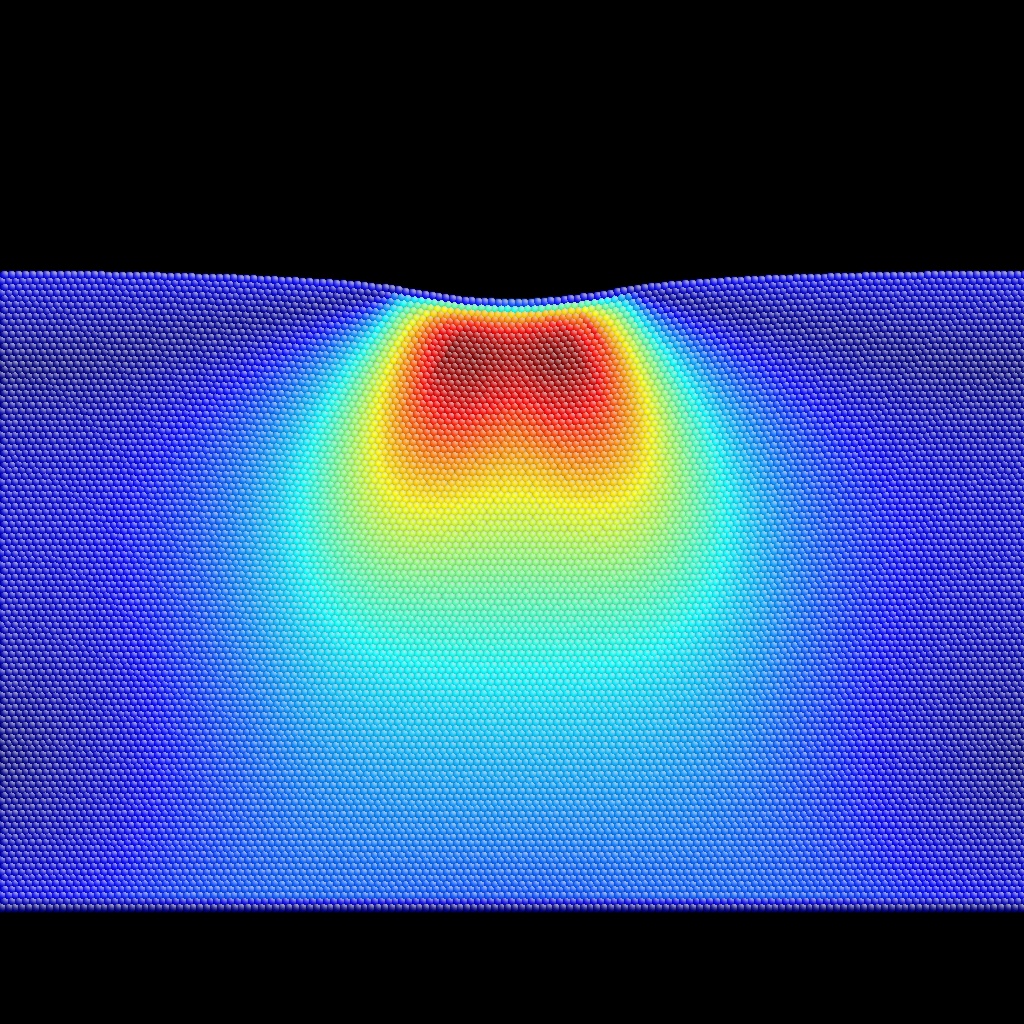
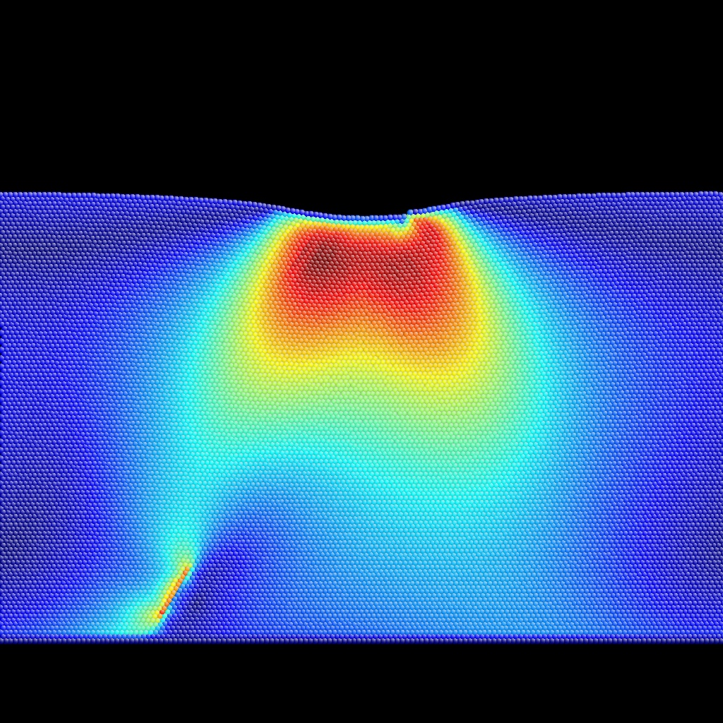
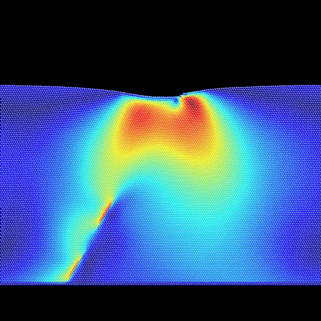
Meta+[0-9,a-f] will color-encode auxiliary properties 0 to 15, whereas Meta+[0-9,a-f] with CapsLock ON will color-encode auxiliary properties 16 to 31. See BubbleRaftBefore.cfg,
BubbleRaftBefore.jpg,
BubbleRaftAfter1.cfg,
BubbleRaftAfter1.jpg,
BubbleRaftAfter2.cfg,
BubbleRaftAfter2.jpg
as examples of input (extended CFG format)
and output for auxiliary property coloring.
Press 'Meta+-','Meta+=','Meta+M' to change the colormaps (available: jet, hot, cool, gray, pink, bone, copper, autumn,
spring, winter, summer,
hsv). Gradation in color only happens for
atoms whose property values are between the lower threshold and the
upper threshold (corresponding to colormap scales 0 and 1,
respectively). Atoms whose property values are outside of the two
thresholds will be rendered invisible by default. This default
behavior can be toggled by pressing 'Ctrl+A', in which case those
atoms whose property values are outside of the thresholds will be
visible but drawn in saturated colors corresponding to colormap scales
0 and 1.
Initially, the upper threshold is taken to be the maximum of the
atoms' auxiliary property values and the lower threshold is taken to
be the minimum. Shift+PageUp will increase the upper threshold,
Shift+PageDown will decrease the upper threshold. Ctrl+PageUp will
increase the lower threshold, Ctrl+PageDown will decrease the lower
threshold. This in turn controls which atoms are drawn and which atoms
are invisible in the default mode. You may also use Shift+T to type in
the thresholds manually. If you wish to recover the initial threshold
values, press 'Ctrl+R'.
When you reload a configuration or make a movie using animation script, the default threshold
behavior is "floating", meaning the program reestablishes the
thresholds for every new config according to the new minimum and
maximum. If you do not want this behavior, pressing 'Ctrl+T' will
toggle to a mode whereby the thresholds remain fixed, or "rigid".
The coloring of atoms can be restored to normal values (of chemical
species) with invisibilities removed by pressing 'o'.
If you make screenshot in eps or jpg or png, there will an
eps file
saved for the color scale, with numerical value labels.
One can assign arbitrary colors and radii to atoms and bonds by
putting a '.usr' patch file with the same name in the same directory
as the '.cfg' file. See for example the file combination Cu.cfg | Cu.usr. This gives ultimate control of
rendering spheres and cylinders to the user. This '.usr' file should
consists of lines that contain either 1, 3, 4, 5, or 6 numbers. The
6-numbers line describes bonds, the rest describes atoms.
A 6-numbers line like
A 5-numbers line like
A 1-number line
The '.usr' patch file will be automatically loaded and applied when
one presses 'Insert'/'Delete' to advance config
list Ctrl+Shift+Right-click will make a certain species or coordination
numbered atoms invisible. Also, when prompted to enter atom color RGB
(see change atom color and/or
radius), '-1 0 0' will make it invisible.
When CapsLock is at On or Meta key is pressed,
right-clicking on a particular atom will make it invisible.
The coloring of atoms can be restored to normal values (of chemical
species) with invisibilities removed by pressing 'o'.
When CapsLock is at On or Meta key is pressed,
right-clicking on a particular bond will make it invisible.
The coloring of bonds can be restored to normal values with
invisibilities removed by pressing 'o'.
Ctrl+Shift+Left-click will prompt the user to change the RGB color
and/or radius of atoms of a certain chemical species, as follows:
If you press Return after being prompted, the values would remain
identical and nothing happens. If you enter one number and Return, it
will be interpreted as the new radius in Angstrom. If you enter three
numbers and Return, it will be interpreted as the new color. Of
course, you can enter all four numbers, in which case the first three
numbers will be taken as the new color.
This link
may help you pick a new color. You may directly enter "255 250 250"
instead of converting them to floating numbers ("1.0 0.98 0.98") first.
When CapsLock is at On or Meta key is pressed,
left-clicking on a particular atom will prompt the user to change its
RGB color and/or radius instead of the whole species.
The coloring of atoms can be restored to normal values (of chemical
species) with invisibilities removed by pressing 'o'.
When CapsLock is at On or Meta key is pressed,
left-clicking on a particular bond
will prompt the user to change the RGB color
and/or radius of the particular bond, as follows:
If you press Return after being prompted, the values would remain
identical and nothing happens. If you enter one number and Return, it
will be interpreted as the new radius in Angstrom. If you enter three
numbers and Return, it will be interpreted as the new color. Of
course, you can enter all four numbers, in which case the first three
numbers will be taken as the new color.
This link
may help you pick a new color. You may directly enter "255 250 250"
instead of converting them to floating numbers ("1.0 0.98 0.98")
first.
The coloring of bonds can be restored to normal values with
invisibilities removed by pressing 'o'.
As a last resort, the user can use
'.usr' file to completely redefine what bonds are drawn, their colors
and radii.
Shift + mouse drag to shift object under PBC. Alternatively, when
CapsLock is at On, Left, Right, Up, Down, Shift+Up, Shift+Down will do
equivalent things as in shift object, except
now in PBC. Lastly, Shift+IMWheel (or Shift+Ctrl+IMWheel for quicker
action) will shift object under PBC in the forward/backward direction.
Press 'z' to recover the initial PBC state, where there is no
shift.
Press 'd', xterm will pop out with inquiry,
Shift+Home/End changes the total view angle that the viewport
spans. The smaller it is, the larger the image appears on screen.
When the session starts, the total span of view is 60 degrees.
Occasionally you want another perspective on the same configuration.
Press 'F4' to new a viewport where all parameters take default
values. Press 'c' to clone a viewport that is exactly the same as the
current one. Press 'q' to quit a certain viewport and free its memory.
Press 's' to print out system status.
Press 'f' to locate an atom by entering its index (0 to
number_of_particles-1). The anchor will
then be set on that atom, and by pulling
closer/away it will be quickly obvious which atom it is.
Press 'g' to go to certain position, maybe somewhere inside the
box, by entering three reduced coordinates.
Just dragging the corner of the window will do, but for more
precise control using terminal input, press 'Ctrl+S'. The recommended
sizes are 320x240, 640x480, 800x600, 1024x1024 ... for certain video
compressors.
Press 'j' to make .jpg screenshot.
Press 'p' to make .png screenshot.
Press 'e' to make high-resolution .eps screenshot (try scale & print).
Press 'v' to toggle auto-invoking shell viewer for screenshots. 'xv', 'ghostview', 'gv' are some of
the applications AtomEye tries to find under the current PATH.
Press 'F9' to load in new config file.
Press 'F10' to reload the config file, in case it has
been refreshed in the meantime.
AtomEye tries to compile a list of config files sequentially
similar to the current config. For example, if we are viewing
"a005.cfg", AtomEye will automatically line up "a000.cfg", "a001.cfg",
.. in front "a005.cfg", and "a006.cfg", "a007.cfg", ... after
"a005.cfg", if these files indeed exist.
Press 'Insert' to backtrack config list and 'Delete' to advance
config list. Press 'Ctrl+Insert' to go to the first of the config list
and 'Ctrl+Delete' to go to the last of the config list. Loop-back is
supported at the two terminations. Press 'Ctrl+F12' to change the
stepping of advance/backtrack; the default stepping is 1.
Press 'F2' to (re)define color tiling blocks. Then, sometime later
on (after a new config has been loaded, see for instance Sequential Config List Browsing), press 'F3' to
show the atoms in previously allocated block colors - be mindful,
however, that the later configurations must have the same number of
atoms as the previous configuration when the color blocks are
defined. If you no longer need to trace anymore, you can free this
extra piece of coloring memory by 'Ctrl+F2'.
'Shift+[0-9,a-f]' will toggle one of the 16 available cutting
planes. The most recently activated cutting plane also gains the
focus. The focused cutting plane can be advanced/retracted by
'Shift+RightArrow/LeftArrow', its sense can be flipped by 'Shift+P',
and it can be deleted from memory by 'Shift+Meta+[0-9,a-f]'.
A cutting planes is created when being toggled for the first
time. The user will be asked to supply six numbers: dx,dy,dz,s0,s1,s2,
where (dx,dy,dz) is the normal vector (doesn't have to normalized) of
the cutting plane in Cartesian frame, (s0,s1,s2) is a point on the
plane in reduced coordinates from 0 to 1. By default dx=1,dy=1,dz=1,
which means the 111 plane, and (s0,s1,s2) is the current anchor position. Usually the user just needs
to input three numbers dx,dy,dz.
There are three ways to input dx,dy,dz,s0,s1,s2:
You can shift an activated cutting plane to the current anchor
position by 'Shift+Ctrl+[0-9,a-f]'.
Besides filtering the atoms, the cutting planes are also
represented by wireframes of their sections with the H-box. A focused
cutting plane's wireframe's color can toggled down to invisible by
'Shift+I'.
To create a dislocation or a crack at the desired place and
inclination, it is usually the easiest to identity two adjacent
crystallographic planes, and apply a force or displacement dipole. To
identify the atoms involved in this operation, first create a cutting plane by for instance pressing
'Shift+0' on FCC10x10x10.cfg. Then,
you need to click on three atoms sequentially on the exposed surface
(to visualize the atoms you click, you may have CapsLock 'on'), and
then press ';'
You will be prompted:
The defaults are generally OK for selecting two atomic planes in
fcc Cu with (111) interplanar spacing 2.0871 Angstrom. Press return
and you will then see:
Your favorite MD or conjugate gradient code can then load in this
"FCC10x10x10.idx" file and have some fun moving these selected atoms.
Before you quit, you may identify the Burgers vector as well by inquiring geometrical info.
Some environments forbid the use of Meta or Alt key. In those
cases, having CapsLock at "on" works as if the Meta key is pressed.
PageDown (Windows) = fn + downarrow (Mac)
Delete (Windows) = fn + delete (Mac)
Insert (Windows) = shift + fn + delete (Mac), or
Insert (Windows) = \ (Mac)
Answer: Try adding
Answer: If you save the screenshot by pressing 'j' or 'p' or
'e', there should be an extra colorbar file saved in .eps with
numerical labels.
Answer: The above error message means some atoms in the
configuration are getting too close to each other. The number of atoms
within the default cutoff radii of first-nearest-neighbors exceeds
24. This usually means there is some pathology in the configuration
(maybe you have miscalculated the atomic geometry? maybe your
time-integrator has blown up?).
To see what is in the configuration, artificially scale up your
supercell 10 times by adding one
optional line after the 'Number of particles = ' line:
Gradually it was realized that X-Window does not provide sufficient native
capability. There are two options. One is to program in OpenGL, the other is to basically
rewrite the graphics functionality of Xlib starting from scratch
(antialised lines, clipping, tilted ellipses, etc.) and just to use X-Window as a pipe (MIT-SHM extension /
XPutImage). I took the second approach based on the observation that
one needs to render very few types of objects in massive
quantities: spheres (as atoms), cylinders (as bonds), and points (as
charge density). Therefore very efficient routines, such as sphere
caching, can be written, which is included in the libAX (Advanced
X) library. Graphics card has
evolved, but so has CPU / main memory, as they essentially are from
the same technology. Therefore in foreseeable future, it is highly
unlikely that this approach loses to OpenGL which depends on polygon
assemblage.
In addition to libAX, a crucial element of AtomEye is the
order-N treatment of atomistic configurations for bond calculation and
coordination number / local strain coloring of atoms. This library,
libAtoms, is shared between AtomEye and an order-N MD code. We
assume always that the configuration is under periodic boundary
condition (PBC) in a parallelepiped box. The rationale is that it is
not too difficult to represent a non-PBC configuration as a PBC
configuration, but not the other way around.
AtomEye was first compiled in 1999, the executable is called A. The early users are myself, Dongyi Liao, Wei
Cai, Dongsheng Xu, Jinpeng Chang and Shigenobu Ogata. Extensive
debugging and improvements have been made to the code, driven by user
requests. AtomEye's screenshots have appeared on the cover of Nature
Materials,
PNAS and
Physical
Review Letters.
Protein Data
Bank format
This format is widely used for storing atomic structure. Its
specifications can be found
here. The standard renderer of PDB file is Rasmol.
HEADER  500 MUST_PBC
CRYST1   13.303   37.627    7.681  60.00  70.00  80.00 P 1           1
in which the first line is a secret code that stays; the
second line contains six numbers,
which should be modified accordingly. The box edges are taken to be
h1=(u1,0,0), h2=(u2,u3,0), h3=(u4,u5,u6) in
Cartesian coordinates, with u1,u2,u3,u4,u5,u6 having one to one
correspondence with a,b,c,alpha,beta,gamma. This connection is
important because the atom positions will be specified in Cartesian
coordinates, so one must unequivocally specify the three PBC edges in
Cartesian coordinates too, fixing the rotational degrees of freedom.
Standard CFG format
Number of particles = 1727
# (required) this must be the first line
A = 1.0 Angstrom (basic length-scale)
# (optional) basic length-scale: default A = 1.0 [Angstrom]
H0(1,1) = 32.5856986704313 A
H0(1,2) = 0 A
H0(1,3) = 0 A
# (required) this is the supercell's 1st edge, in A

H0(2,1) = 8.64689152483509e-16 A
H0(2,2) = 32.5856986704313 A
H0(2,3) = 0 A
# (required) this is the supercell's 2nd edge, in A

H0(3,1) = 8.64689152483509e-16 A
H0(3,2) = 8.64689152483509e-16 A
H0(3,3) = 32.5856986704313 A
# (required) this is the supercell's 3rd edge, in A
Transform(1,1) = 1
Transform(1,2) = 0
Transform(1,3) = 0
Transform(2,1) = 0
Transform(2,2) = 1
Transform(2,3) = 0
Transform(3,1) = 0
Transform(3,2) = 0
Transform(3,3) = 1
# (optional) apply additional transformation on H0:  H = H0 * Transform;
# default = Identity matrix.

eta(1,1) = 0
eta(1,2) = 0
eta(1,3) = 0
eta(2,2) = 0
eta(2,3) = 0
eta(3,3) = 0
# (optional) apply additional Lagrangian strain on H0:
# H = H0 * sqrt(Identity_matrix + 2 * eta);
# default = zero matrix.
# ENSUING ARE THE ATOMS, EACH ATOM DESCRIBED BY A ROW
# 1st entry is atomic mass in a.m.u.
# 2nd entry is the chemical symbol (max 2 chars)

# 3rd entry is reduced coordinate s1 (dimensionless)
# 4th entry is reduced coordinate s2 (dimensionless)
# 5th entry is reduced coordinate s3 (dimensionless)
# real coordinates x = s * H,  x, s are 1x3 row vectors

# 6th entry is d(s1)/dt in basic rate-scale R
# 7th entry is d(s2)/dt in basic rate-scale R
# 8th entry is d(s3)/dt in basic rate-scale R
R = 1.0 [ns^-1]
# (optional) basic rate-scale: default R = 1.0 [ns^-1]
28.0855 Si .0208333333333333 .0208333333333333 .0208333333333333 0 0 0
28.0855 Si .0625 .0625 .0625 0 0 0
28.0855 Si .0208333333333333 .104166666666667 .104166666666667 0 0 0
28.0855 Si .0625 .145833333333333 .145833333333333 0 0 0
28.0855 Si .104166666666667 .0208333333333333 .104166666666667 0 0 0
28.0855 Si .145833333333333 .0625 .145833333333333 0 0 0
....
 x  =  s1 * H(1,1)  +  s2 * H(2,1)  +  s3 * H(3,1)
 y  =  s1 * H(1,2)  +  s2 * H(2,2)  +  s3 * H(3,2)
 z  =  s1 * H(1,3)  +  s2 * H(2,3)  +  s3 * H(3,3)
Extended CFG format
Number of particles = 16200
A = 4.37576470588235 Angstrom (basic length-scale)
H0(1,1) = 127.5 A
H0(1,2) = 0 A
H0(1,3) = 0 A
H0(2,1) = 0 A
H0(2,2) = 119.501132067411 A
H0(2,3) = 0 A
H0(3,1) = 0 A
H0(3,2) = 0 A
H0(3,3) = 3 A
.NO_VELOCITY.
entry_count = 11
auxiliary[0] = kine [reduced unit]
auxiliary[1] = pote [reduced unit]
auxiliary[2] = s11 [reduced unit]
auxiliary[3] = s22 [reduced unit]
auxiliary[4] = s12 [reduced unit]
auxiliary[5] = hydro [reduced unit]
auxiliary[6] = mises [reduced unit]
auxiliary[7] = Lmin [reduced unit]
1.000000
Ar
0.005 0.01232 0.5 0 -2.9819 0.79705 2.3326 0.022255 1.5648 0.76808 102.82
....
28.0855
Si
0.005 0.01232 0.5 0 -2.9819 0.79705 2.3326 0.022255 1.5648 0.76808 102.82
12.011
C
0.091667 0.01232 0.5 0 -2.9491 1.3535 3.9801 0.9655 2.6668 1.63 103.07
28.0855
Si
0.31833 0.01232 0.5 0 -2.9787 0.84615 2.4817 0.45222 1.6639 0.93449 103.02
12.011
C
0.765 0.01232 0.5 0 -2.9431 1.4263 4.1825 -1.0568 2.8044 1.7367 102.97
which takes up no more space than the standard CFG format under
UNIX. Of course a space-saving way is to write the above as,
28.0855
Si
0.005 0.01232 0.5 0 -2.9819 0.79705 2.3326 0.022255 1.5648 0.76808 102.82
0.31833 0.01232 0.5 0 -2.9787 0.84615 2.4817 0.45222 1.6639 0.93449 103.02
12.011
C
0.091667 0.01232 0.5 0 -2.9491 1.3535 3.9801 0.9655 2.6668 1.63 103.07
0.765 0.01232 0.5 0 -2.9431 1.4263 4.1825 -1.0568 2.8044 1.7367 102.97
102.54352   3.781
-54.324521 -9.035
22.870594   0.785
-9.8543543  6.834
....
where each line contains the property values for one atom, and the
total number of lines is equal to the total number of atoms. An
example would be amorphous_Si.cfg
| amorphous_Si.aux file
combination. See auxiliary
property coloring for how the coloring intensity is controlled.
Manual
Usage:
Download binary from browser and save as A
You must ensure that the "xterm" command is in your shell PATH and can
be directly called. See also here
if your configuration file has been compressed.
NumLock:
In general, your NumLock key should be in the 'off' state. Otherwise,
AtomEye will regard it as equivalent to having CapsLock 'on', which is
equivalent to having Meta+ modifier for every key
you press.
Help Key:
Press 'F1' or 'h' for help.
Rotate Object (or so you think):
Anchor Control:
Toggle Bond Mode:
Toggle Between Parallel / Perspective Projection:
Scale Atom Radii:
Change Bond Radius:
Toggle Wireframe Mode:
Cutoff Control:
Make Viewframe Upright:
Inquire Atom Information:
Inquire Geometrical Information:
Pull Viewport Closer/Away from the Anchor:
Shift Object (or so you think):
Changing Gearbox Value:
[1]0.001 [2]0.002 [3]0.005 [4]0.010 [5]0.020
[6]0.050 [7]0.100 [8]0.200 [9]0.500 [0]0.150
The gearbox value controls all rate of change, such as angle of
rotation, amount of translation, the rate of atom radius change, etc.
Coordination Number Coloring:
Atomistic Local von Mises Shear Strain Invariant Coloring:
Central Symmetry Parameter
Coloring:
Least-Square Atomic Local Strain Tensor Coloring:
We have implemented atomic
local strain tensor coloring as a core functionality of AtomEye
(please cite F. Shimizu, S. Ogata and J. Li, "Theory of Shear Banding in
Metallic Glasses and Molecular Dynamics Calculations,"
Materials Transactions 48 (2007) 2923-2927, if you use
this characterization). It is different from the von Mises shear strain invariant
coloring in that two configurations are required, one current, and
one reference configuration. It is also much more powerful and robust
than the former because it does not rely on assumptions of prior high
lattice symmetry.
dx_{ij}(now) \approx dx_{ij}(reference) J
where dx's are row vectors, and j are i's nearest neighbors (in the present
configuration, as we don't want to store two neighborlists).
Auxiliary Property
Coloring:
Apply Extra Color Patch:
0 3 0 1 0 0.2
would mean drawing a bond between atom 0 and atom 3, with bond color
"0 1 0" and radius 0.2. Note that atom index in AtomEye
starts from 0 as in C language
convention (that is, the first atom in the cfg file has index 0).
2 0 1 0 0.7
would mean drawing atom 2 with color "0 1 0" and radius 0.7
0.7
or a 3-numbers line
0 1 0
or a 4-numbers line
0 1 0 0.7
would mean drawing atom m with radius 0.7 (with default color),
color "0 1 0" (with default radius), or color "0 1 0" and radius 0.7,
respectively.
m will be automatically accumulated, starting from 0.
Make Atoms Invisible:
Make Bond Invisible:
Change Atom Color and/or Radius:
Change color [radius] of type-3 ("P") atoms (0.100 0.700 0.300 [1.060]):
The first three numbers are the RGB values of Phosphorus.
The last number in the square bracket is its radius (currently taken
to be the charge
radius, another alternative is the empirical
atomic radius) in Angstrom. The rendered radius is the above
scaled by a common factor (scale atom
radii).
Change Bond Color and/or Radius:
Change color [radius] of bond-1726 (0.493 0.493 0.561 [0.250]):
The first three numbers are the RGB values of the bond. The last
number in the square bracket is its radius in Angstrom.
Shift object under PBC:
Change Background Color:
Change background color (0.000 0.000 0.000):
and you should input three real numbers from 0 to 1 for the RGB
values. If you press Return, the numbers in the brackets will
be taken as the input. They are just the current background colors,
so nothing will change.
Change View Angle Amplification:
New, Clone, Quit Viewport:
Print System Status:
Find an Atom:
Go to Position:
Resize Window
Making jpeg Screenshot:
Making png Screenshot:
Making Encapsulated PostScript Screenshot:
Toggle Auto-Invoking Shell Viewer:
Load New Config:
Reload Configuration:
Sequential Config List Browsing:
Define and Trace Color Tiling Blocks:
Creating and Manipulating Cutting Planes
Save Atom Indices in a File
Interplanar spacing [A] z-margin [A] xy-tolerance (2.5 0.01 0.01):
down=4 and up=1 atoms selected in filter.
Save the selected atoms to (FCC10x10x10.idx):
selected atom indices [0-31999] saved to FCC10x10x10.idx.
which means 4 atoms in the "down" plane and 1 atom in the "up" plane
are selected, and the atom indices (remember that AtomEye always
counts from 0) are saved in "FCC10x10x10.idx", which looks like:
% more FCC10x10x10.idx
4 1
14267
14550
14576
17421
17760
The first 4 indices are atoms on the "down" parallelogram, followed by
the 1 atom on the "up" parallelogram. Note that the "up" direction is
the right-handed rotational axis represented by the three sequentially
clicked atomic positions. In other words, you must click on the "down"
atoms in anti-clockwise fashion. The make sure, you can explicitly check the
printout
"up" is [0.57735 0.57735 0.57735]
check it agrees with your mirror normal...
with your desired "up" direction.
Making movie:
90
00001.cfg Pic/00001.jpg
00002.cfg Pic/00002.jpg
00003.cfg Pic/00003.jpg
00004.cfg Pic/00004.jpg
00005.cfg Pic/00005.jpg
The first integer (from 0 to 100) specifies the quality of the
images. The larger it is, the less the compression and the better
the quality. Usually 90 is very good and 80 is good enough. Rows
of string pairs then follow. The first string is the input
configuration filename. The second string is the output image
filename. Depending on the suffix, .jpg,
.png, or .eps
screenshots will be saved. One can also use absolute
pathnames. It is better to separate the configuration files with
the image files, therefore "Pic/00001.jpg" and so on is
recommended. "scr_anim" itself can be
created for example by using the following Matlab script create_scr_anim.m. If "scr_anim" does not exist, AtomEye will offer to
create a default one, in which case .jpg
format is used with quality 90, and the frames will go to the Jpgs/ directory (created by AtomEye if
it doesn't exist already).
What is the Meta key?
Mac Keybinding
PageUp (Windows) = fn + uparrow (Mac)
Binary Release
These are raw binaries. Right-click on the link and "Save Target
As..." to one of your directories. Then run "chmod 755" on the
file. To test, you need to save a CFG file as well, such as cnt8x3.cfg.
When I get the chance, I try to make up-to-date executables for
different platforms, but only the i686 Linux one is guaranteed
to be of the latest stable version with full functionality.
Frequently Asked Questions
export XLIB_SKIP_ARGB_VISUALS=1
to your .bashrc file.
ATOM_COORDINATION_MAX = 24 exceeded
or
error: Imakespace: min=0 max=2744 jammed between i=1262 and i+1.
and AtomEye quits. What's the problem?
A = 10 Angstrom (basic length-scale)
Most likely this would reduce all atoms to coordination-0. But at
least you can now load your configuration into AtomEye, see the atoms,
and debug the configuration.
Bug report
There will always be bugs in AtomEye. When you think you have
encountered one, please do the following:
History
I started using Rasmol in
1997 and was quite impressed. But its as well as PDB file format's limitations for
large-scale molecular dynamics (MD) simulations became painfully
obvious after some time. My colleagues Dongyi Liao, Wei Cai and myself
all started developing our own molecular visualization codes. It was a
very friendly and helpful environment even though we differ in coding
styles, and a lot of ideas were exchanged. Some of my earlier attempts
are placed here.